結論としては、相手が投手王国なら

0アウト1塁 →　1アウト2塁にするのは効果的だと思う

データの取得、まとめがあってれば。

今回は備忘録や検証用でコードを残す意味合い

データ取得

pybaseballというライブラリをインストールし、その後にstatcast関数を用いて、2022年のメジャーリーグベースボールのデータを取得しています。

!pip install pybaseball
from pybaseball import statcast
df = statcast(start_dt='2022-03-31', end_dt='2022-12-31')

0アウトランナー1塁(2022)

ノーアウトランナー1塁・送りバント後に得点がつながった割合

このコードでは、送りバントが行われたプレイを分析して、送りバント後に得点がつながった割合を計算します。まず、アウトが0で1塁ランナーがいる状況をフィルタリングし、df_filteredというデータフレームに格納します。

次に、sac_buntイベントであるプレイを抽出し、sac_buntsという新しいデータフレームにコピーします。これにより、送りバントが行われたプレイを独立して分析できます。

そして、各送りバント後にそのイニングで得点がつながったかどうかを調べ、inning_scoresというリストに結果を格納します。同じイニングで同じチームのすべてのプレイを取得し、得点が記録されたかどうかを確認します。得点が記録された場合、runs_scoredにTrueが格納されます。

その後、sac_buntsデータフレームにinning_scoredという新しい列を追加し、各送りバントが得点につながったかどうかを格納します。そして、得点につながった送りバントの割合を計算し、percentage_scoredに格納します。

最後に、送りバントが行われた回数と、送りバント後に得点がつながった回数を表示し、送りバントが行われた後、その回に得点がつながった割合を計算して表示します。



# Filter for plays with no outs and a runner on first base
df_filtered = df[(df['outs_when_up'] == 0) & (df['on_1b'].notna()) & (df['on_2b'].isna()) & (df['on_3b'].isna())]

# Filter for sacrifice bunt events
sac_bunts = df_filtered[df_filtered['events'] == 'sac_bunt'].copy()

# Check whether a run was scored in the same inning after the sac bunt
inning_scores = []
for index, row in sac_bunts.iterrows():
    inning = row['inning']
    game_pk = row['game_pk']
    inning_topbot = row['inning_topbot']
    
    # Get all plays in the same inning for the same team
    same_inning_plays = df[(df['game_pk'] == game_pk) & (df['inning'] == inning) & (df['inning_topbot'] == inning_topbot)].copy()
    
    # Check if any runs were scored
    same_inning_plays['scored'] = same_inning_plays['post_home_score'] - same_inning_plays['home_score'] + same_inning_plays['post_away_score'] - same_inning_plays['away_score']
    runs_scored = (same_inning_plays['scored'] > 0).any()
    
    inning_scores.append(runs_scored)

sac_bunts['inning_scored'] = inning_scores

# Calculate the percentage of sac bunts that led to a run being scored
percentage_scored = sac_bunts['inning_scored'].mean() * 100

# Count the number of sac bunts and the number of times a run was scored after a sac bunt
total_sac_bunts = len(sac_bunts)
scored_after_sac_bunt = sac_bunts['inning_scored'].sum()

print(f"送りバントが行われた回数は {total_sac_bunts} 回です。")
print(f"送りバント後に得点がつながった回数は {scored_after_sac_bunt} 回です。")
print(f"送りバントが行われた後、その回に得点がつながった割合は {percentage_scored:.2f}% です。")

結果

送りバントが行われた回数は 156 回です。
送りバント後に得点がつながった回数は 65 回です。
送りバントが行われた後、その回に得点がつながった割合は 41.67% です。

ノーアウトランナー1塁・送りバントが行われなかった場合に得点がつながった割合

このコードでは、送りバント以外のプレイを分析して、送りバントが行われなかった場合に得点がつながった割合を計算します。まず、sac_buntイベント以外のプレイを抽出し、non_sac_buntsという新しいデータフレームにコピーします。これにより、送りバント以外のプレイを独立して分析できます。

そして、各送りバント以外のプレイ後にそのイニングで得点がつながったかどうかを調べ、inning_scores_non_sacというリストに結果を格納します。同じイニングで同じチームのすべてのプレイを取得し、得点が記録されたかどうかを確認します。得点が記録された場合、runs_scoredにTrueが格納されます。

その後、non_sac_buntsデータフレームにinning_scoredという新しい列を追加し、各送りバント以外のプレイが得点につながったかどうかを格納します。そして、得点につながった送りバント以外のプレイの割合を計算し、percentage_scored_non_sacに格納します。

最後に、送りバント以外のプレイが行われた回数と、送りバント以外のプレイ後に得点がつながった回数を表示し、送りバントが行われなかった後、その回に得点がつながった割合を計算して表示します

# Filter for non-sacrifice bunt events
non_sac_bunts = df_filtered[df_filtered['events'] != 'sac_bunt'].copy()

# Check whether a run was scored in the same inning without a sac bunt
inning_scores_non_sac = []
for index, row in non_sac_bunts.iterrows():
    inning = row['inning']
    game_pk = row['game_pk']
    inning_topbot = row['inning_topbot']
    
    # Get all plays in the same inning for the same team
    same_inning_plays = df[(df['game_pk'] == game_pk) & (df['inning'] == inning) & (df['inning_topbot'] == inning_topbot)].copy()
    
    # Check if any runs were scored
    same_inning_plays['scored'] = same_inning_plays['post_home_score'] - same_inning_plays['home_score'] + same_inning_plays['post_away_score'] - same_inning_plays['away_score']
    runs_scored = (same_inning_plays['scored'] > 0).any()
    
    inning_scores_non_sac.append(runs_scored)

non_sac_bunts['inning_scored'] = inning_scores_non_sac

# Calculate the percentage of non-sac bunts that led to a run being scored
percentage_scored_non_sac = non_sac_bunts['inning_scored'].mean() * 100

# Count the number of non-sac bunts and the number of times a run was scored without a sac bunt
total_non_sac_bunts = len(non_sac_bunts)
scored_after_non_sac_bunt = non_sac_bunts['inning_scored'].sum()

print(f"バントを行わなかった回数は {total_non_sac_bunts} 回です。")
print(f"バントを行わなかった後に得点がつながった回数は {scored_after_non_sac_bunt} 回です。")
print(f"バントを行わなかった後、その回に得点がつながった割合は {percentage_scored_non_sac:.2f}% です。")

結果

バントを行わなかった回数は 39025 回です。
バントを行わなかった後に得点がつながった回数は 17494 回です。
バントを行わなかった後、その回に得点がつながった割合は 44.83% です

各チームの結果・ノーアウトランナー1塁・送りバント有無での得点

このコードでは、各チームの送りバントが行われた場合と送りバントが行われなかった場合に、それぞれ得点がつながった割合を計算し、チームごとの結果を表示します。

まず、teamsという変数にユニークなチームのリストを取得します。次に、各チームについて、送りバントが行われた場合と送りバントが行われなかった場合の得点がつながった割合を計算します。この計算は、ホームチームとアウェイチームの両方に適用され、攻撃が裏で行われるホームチームと表で行われるアウェイチームに対応しています。

各チームの送りバント後の得点割合と送りバント以外のプレイ後の得点割合を計算したら、team_scoresというリストに結果を格納します。このリストは、チーム名、送りバント後の得点割合、送りバント以外のプレイ後の得点割合を含む辞書で構成されています。

最後に、team_scoresリストをデータフレームに変換し、team_scores_dfという変数に格納します。そして、このデータフレームを表示して、各チームの送りバント後と送りバント以外のプレイ後の得点割合を確認できます。

# 攻撃は、home_team は　裏に攻撃します。away_team は、表に攻撃します。
# 守備は、home_team は　表に守備をします。away_team は、裏に守備をします。

import pandas as pd

team_scores = []

# Get the unique list of teams
teams = df_filtered['home_team'].unique()

for team in teams:
    # Filter for sac bunt events for the team
    sac_bunts_team = sac_bunts[((sac_bunts['home_team'] == team) & (sac_bunts['inning_topbot'] == 'Bot')) | ((sac_bunts['away_team'] == team) & (sac_bunts['inning_topbot'] == 'Top'))]
    
    # Calculate the percentage of sac bunts that led to a run being scored
    percentage_scored_sac_team = sac_bunts_team['inning_scored'].mean() * 100
    
    # Filter for non-sac bunt events for the team
    non_sac_bunts_team = non_sac_bunts[((non_sac_bunts['home_team'] == team) & (non_sac_bunts['inning_topbot'] == 'Bot')) | ((non_sac_bunts['away_team'] == team) & (non_sac_bunts['inning_topbot'] == 'Top'))]
    
    # Calculate the percentage of non-sac bunts that led to a run being scored
    percentage_scored_non_sac_team = non_sac_bunts_team['inning_scored'].mean() * 100
    
    team_scores.append({
        'team': team,
        'sac_bunt_percentage': percentage_scored_sac_team,
        'non_sac_bunt_percentage': percentage_scored_non_sac_team
    })

team_scores_df = pd.DataFrame(team_scores)

print(team_scores_df)

結果

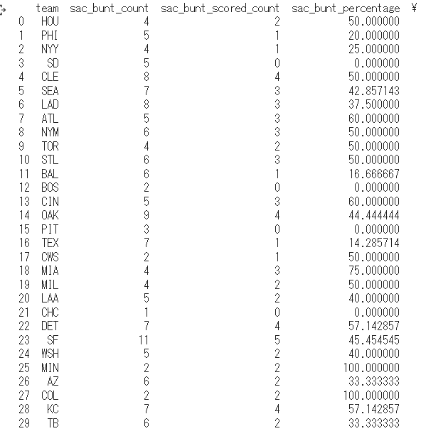
各チームの結果・ノーアウトランナー1塁・送りバント有無での得点(回数も表示)

このコードでは、各チームの送りバントが行われた場合と送りバントが行われなかった場合に、それぞれ得点がつながった割合だけでなく、送りバントおよび送りバント以外のプレイが行われた回数と、それらが得点につながった回数も計算して表示します。

まず、各チームについて送りバントが行われた場合の得点割合を計算し、送りバントが行われた回数と得点につながった回数を求めます。同様に、各チームについて送りバントが行われなかった場合の得点割合を計算し、送りバント以外のプレイが行われた回数と得点につながった回数を求めます。

次に、各チームの送りバント回数、送りバント後に得点がつながった回数、送りバント後の得点割合、送りバント以外のプレイ回数、送りバント以外のプレイ後に得点がつながった回数、送りバント以外のプレイ後の得点割合を辞書に格納します。この辞書は、team_scoresというリストに追加されます。

最後に、team_scoresリストをデータフレームに変換し、team_scores_dfという変数に格納します。そして、このデータフレームを表示して、各チームの送りバント回数、送りバント後に得点がつながった回数、送りバント後の得点割合、送りバント以外のプレイ回数、送りバント以外のプレイ後に得点がつながった回数、送りバント以外のプレイ後の得点割合を確認できます。

team_scores = []

for team in teams:
    # Filter for sac bunt events for the team
    sac_bunts_team = sac_bunts[((sac_bunts['home_team'] == team) & (sac_bunts['inning_topbot'] == 'Bot')) | ((sac_bunts['away_team'] == team) & (sac_bunts['inning_topbot'] == 'Top'))]
    
    # Calculate the percentage of sac bunts that led to a run being scored
    percentage_scored_sac_team = sac_bunts_team['inning_scored'].mean() * 100
    
    # Calculate the number of sac bunts and the number of times they led to a run being scored
    sac_bunt_count = len(sac_bunts_team)
    sac_bunt_scored_count = sac_bunts_team['inning_scored'].sum()
    
    # Filter for non-sac bunt events for the team
    non_sac_bunts_team = non_sac_bunts[((non_sac_bunts['home_team'] == team) & (non_sac_bunts['inning_topbot'] == 'Bot')) | ((non_sac_bunts['away_team'] == team) & (non_sac_bunts['inning_topbot'] == 'Top'))]
    
    # Calculate the percentage of non-sac bunts that led to a run being scored
    percentage_scored_non_sac_team = non_sac_bunts_team['inning_scored'].mean() * 100
    
    # Calculate the number of non-sac bunts and the number of times they led to a run being scored
    non_sac_bunt_count = len(non_sac_bunts_team)
    non_sac_bunt_scored_count = non_sac_bunts_team['inning_scored'].sum()
    
    team_scores.append({
        'team': team,
        'sac_bunt_count': sac_bunt_count,
        'sac_bunt_scored_count': sac_bunt_scored_count,
        'sac_bunt_percentage': percentage_scored_sac_team,
        'non_sac_bunt_count': non_sac_bunt_count,
        'non_sac_bunt_scored_count': non_sac_bunt_scored_count,
        'non_sac_bunt_percentage': percentage_scored_non_sac_team
    })

team_scores_df = pd.DataFrame(team_scores)

print(team_scores_df)

結果

各チームの送りバントが行われなかった場合の得点割合

このコードでは、各チームの送りバントが行われなかった場合の得点割合を、低い順に並べた棒グラフを描画します。

import matplotlib.pyplot as plt

sorted_df = team_scores_df.sort_values('non_sac_bunt_percentage', ascending=True)

# プロットの準備
fig, ax = plt.subplots(figsize=(15, 7))

# 棒グラフをプロットします。
ax.bar(sorted_df['team'], sorted_df['non_sac_bunt_percentage'], color='blue')

# 軸ラベルとタイトルを設定します。
ax.set_xlabel('Teams')
ax.set_ylabel('score_percentage_without_bunt')
ax.set_title('score_percentage_without_bunt by Team (Low to High)')

# グラフを表示します。
plt.show()

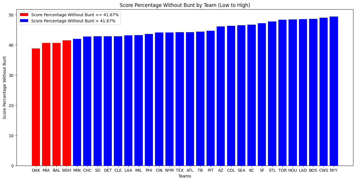
各チームの送りバントが行われなかった場合の得点割合・バント時の得点割合以下を赤

このコードでは、各チームの送りバントが行われなかった場合の得点割合を、低い順に並べた棒グラフを描画し、平均値に基づいて色分けしています。

import matplotlib.pyplot as plt

# データフレームのカラム名を更新します
team_scores_df = team_scores_df.rename(columns={'non_sac_bunt_percentage': 'score_percentage_without_bunt'})

# データフレームを 'score_percentage_without_bunt' で昇順にソートします
sorted_df = team_scores_df.sort_values('score_percentage_without_bunt', ascending=True)

# 色分けのために、'score_percentage_without_bunt' が全体の平均値より大きいかどうかを判断するカラムを追加します
sorted_df['greater_than_average'] = sorted_df['score_percentage_without_bunt'] > percentage_scored

# プロットの準備
fig, ax = plt.subplots(figsize=(15, 7))

# 色分けした棒グラフをプロットします
ax.bar(sorted_df['team'][~sorted_df['greater_than_average']],
       sorted_df['score_percentage_without_bunt'][~sorted_df['greater_than_average']],
       color='red', label=f'Score Percentage Without Bunt <= {percentage_scored:.2f}%')
ax.bar(sorted_df['team'][sorted_df['greater_than_average']],
       sorted_df['score_percentage_without_bunt'][sorted_df['greater_than_average']],
       color='blue', label=f'Score Percentage Without Bunt > {percentage_scored:.2f}%')

# 軸ラベルとタイトルを設定します
ax.set_xlabel('Teams')
ax.set_ylabel('Score Percentage Without Bunt')
ax.set_title('Score Percentage Without Bunt by Team (Low to High)')

# 凡例を表示します
ax.legend()

# グラフを表示します
plt.show()

守備チームから見たバント有無での失点割合

このコードでは、各チームの送りバントおよび非送りバントの状況における得点割合を、守備チームとして集計しています。

まず、チームごとにループを回して、送りバントおよび非送りバントイベントをフィルタリングします。ただし、今回は守備チームとしてフィルタリングを行います。

次に、送りバントイベントの場合、それが得点につながった割合を計算し、送りバントイベントの総数と得点につながった回数も計算します。

同様に、非送りバントイベントの場合、それが得点につながった割合を計算し、非送りバントイベントの総数と得点につながった回数も計算します。

最後に、それぞれのチームごとに集計した値をリストに追加し、最終的なデータフレームを作成して表示します。

team_scores = []

for team in teams:
    # Filter for sac bunt events for the team as the defensive team
    sac_bunts_team = sac_bunts[((sac_bunts['home_team'] == team) & (sac_bunts['inning_topbot'] == 'Top')) | ((sac_bunts['away_team'] == team) & (sac_bunts['inning_topbot'] == 'Bot'))]
    
    # Calculate the percentage of sac bunts that led to a run being scored
    percentage_scored_sac_team = sac_bunts_team['inning_scored'].mean() * 100
    
    # Calculate the number of sac bunts and the number of times they led to a run being scored
    sac_bunt_count = len(sac_bunts_team)
    sac_bunt_scored_count = sac_bunts_team['inning_scored'].sum()
    
    # Filter for non-sac bunt events for the team as the defensive team
    non_sac_bunts_team = non_sac_bunts[((non_sac_bunts['home_team'] == team) & (non_sac_bunts['inning_topbot'] == 'Top')) | ((non_sac_bunts['away_team'] == team) & (non_sac_bunts['inning_topbot'] == 'Bot'))]
    
    # Calculate the percentage of non-sac bunts that led to a run being scored
    percentage_scored_non_sac_team = non_sac_bunts_team['inning_scored'].mean() * 100
    
    # Calculate the number of non-sac bunts and the number of times they led to a run being scored
    non_sac_bunt_count = len(non_sac_bunts_team)
    non_sac_bunt_scored_count = non_sac_bunts_team['inning_scored'].sum()
    
    team_scores.append({
        'team': team,
        'sac_bunt_count': sac_bunt_count,
        'sac_bunt_scored_count': sac_bunt_scored_count,
        'sac_bunt_percentage': percentage_scored_sac_team,
        'non_sac_bunt_count': non_sac_bunt_count,
        'non_sac_bunt_scored_count': non_sac_bunt_scored_count,
        'non_sac_bunt_percentage': percentage_scored_non_sac_team
    })

team_scores_df = pd.DataFrame(team_scores)

print(team_scores_df)

結果

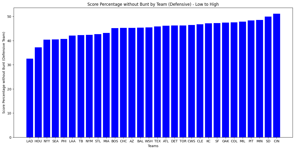
守備チームから見たバント有無・失点の割合(グラフ)

このコードは、各チームの守備時における非送りバントイベントが得点につながった割合をプロットした棒グラフを作成し、表示しています。

import matplotlib.pyplot as plt

sorted_df = team_scores_df.sort_values('non_sac_bunt_percentage', ascending=True)

# プロットの準備
fig, ax = plt.subplots(figsize=(15, 7))

# 棒グラフをプロットします。
ax.bar(sorted_df['team'], sorted_df['non_sac_bunt_percentage'], color='blue')

# 軸ラベルとタイトルを設定します。
ax.set_xlabel('Teams')
ax.set_ylabel('Score Percentage without Bunt (Defensive Team)')
ax.set_title('Score Percentage without Bunt by Team (Defensive) - Low to High')

# グラフを表示します。
plt.show()

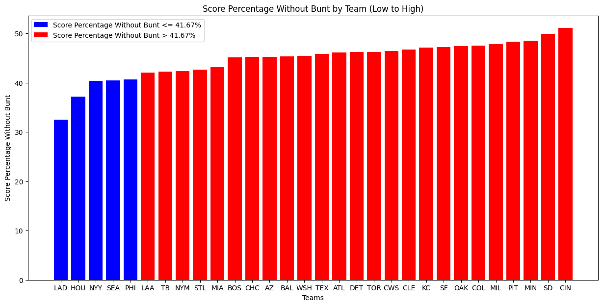
守備チームから見たバント有無・バントでの得点率よりも低いチームを青

LAD チーム防御率高いだけある

import matplotlib.pyplot as plt

# データフレームのカラム名を更新します
team_scores_df = team_scores_df.rename(columns={'non_sac_bunt_percentage': 'score_percentage_without_bunt'})

# データフレームを 'score_percentage_without_bunt' で昇順にソートします
sorted_df = team_scores_df.sort_values('score_percentage_without_bunt', ascending=True)

# 色分けのために、'score_percentage_without_bunt' が全体の平均値より大きいかどうかを判断するカラムを追加します
sorted_df['greater_than_average'] = sorted_df['score_percentage_without_bunt'] > percentage_scored

# プロットの準備
fig, ax = plt.subplots(figsize=(15, 7))

# 色分けした棒グラフをプロットします
ax.bar(sorted_df['team'][~sorted_df['greater_than_average']],
       sorted_df['score_percentage_without_bunt'][~sorted_df['greater_than_average']],
       color='blue', label=f'Score Percentage Without Bunt <= {percentage_scored:.2f}%')
ax.bar(sorted_df['team'][sorted_df['greater_than_average']],
       sorted_df['score_percentage_without_bunt'][sorted_df['greater_than_average']],
       color='red', label=f'Score Percentage Without Bunt > {percentage_scored:.2f}%')

# 軸ラベルとタイトルを設定します
ax.set_xlabel('Teams')
ax.set_ylabel('Score Percentage Without Bunt')
ax.set_title('Score Percentage Without Bunt by Team (Low to High)')

# 凡例を表示します
ax.legend()

# グラフを表示します
plt.show()

1アウトランナー2塁(2022)

得点する割合

このコードは、1アウトで2塁にランナーがいる状況で、同じイニングで得点が記録される確率を計算しています。具体的な手順は以下の通りです。

df_filtered というデータフレームを作成し、1アウトで2塁にランナーがいる状況のプレイデータをフィルタリングして格納します。
各プレイのイニングごとに、そのイニングで得点が記録されたかどうかをチェックし、inning_scores リストに格納します。
inning_scores リストの平均値を計算し、1アウトで2塁にランナーがいる状況で得点が記録される確率（パーセンテージ）を求めます。
結果を表示します。

# Filter for plays with 1 out and a runner on second base
df_filtered = df[(df['outs_when_up'] == 1) & (df['on_1b'].isna()) & (df['on_2b'].notna()) & (df['on_3b'].isna())]


# Check whether a run was scored in the same inning
inning_scores = []
for index, row in df_filtered.iterrows():
    inning = row['inning']
    game_pk = row['game_pk']
    inning_topbot = row['inning_topbot']
    
    # Get all plays in the same inning for the same team
    same_inning_plays = df[(df['game_pk'] == game_pk) & (df['inning'] == inning) & (df['inning_topbot'] == inning_topbot)].copy()
    
    # Check if any runs were scored
    same_inning_plays['scored'] = same_inning_plays['post_home_score'] - same_inning_plays['home_score'] + same_inning_plays['post_away_score'] - same_inning_plays['away_score']
    runs_scored = (same_inning_plays['scored'] > 0).any()
    
    inning_scores.append(runs_scored)

df_filtered['inning_scored'] = inning_scores

# Calculate the percentage of plays from 1 out and a runner on first base that led to a run being scored
percentage_scored = df_filtered['inning_scored'].mean() * 100

# Count the number of plays and the number of times a run was scored
total_plays = len(df_filtered)
scored_from_1_out_2_base = df_filtered['inning_scored'].sum()

print(f"1アウト2塁の状況が {total_plays} 回ありました。")
print(f"1アウト2塁の状況から得点がつながった回数は {scored_from_1_out_2_base} 回です。")
print(f"1アウト2塁の状況から得点がつながった割合は {percentage_scored:.2f}% です。")

結果

1アウト2塁の状況が 19147 回ありました。
1アウト2塁の状況から得点がつながった回数は 10493 回です。
1アウト2塁の状況から得点がつながった割合は 54.80% です。

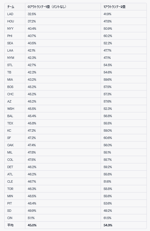
各チームの攻撃での得点割合

このコードは、各チームごとに1アウト2塁の状況が何回あったか、そのうち何回得点がつながったか、そして得点がつながった割合を計算し、それらの情報をデータフレームにまとめて表示します。

import pandas as pd

teams = df['home_team'].unique()

team_scores = []

for team in teams:
    # Filter for 1 out 2 base events for the team
    team_plays = df_filtered[((df_filtered['home_team'] == team) & (df_filtered['inning_topbot'] == 'Bot')) | ((df_filtered['away_team'] == team) & (df_filtered['inning_topbot'] == 'Top'))]
    
    # Calculate the percentage of plays that led to a run being scored
    percentage_scored_team = team_plays['inning_scored'].mean() * 100
    
    # Calculate the number of plays and the number of times they led to a run being scored
    plays_count = len(team_plays)
    plays_scored_count = team_plays['inning_scored'].sum()
    
    team_scores.append({
        'team': team,
        'plays_count': plays_count,
        'plays_scored_count': plays_scored_count,
        'percentage_scored': percentage_scored_team
    })

team_scores_df = pd.DataFrame(team_scores)

print(team_scores_df)

結果、

各チームの攻撃での得点割合(グラフ)

このコードは、各チームごとの1アウト2塁の状況で得点がつながった割合を、昇順にソートした棒グラフで表示します。

import matplotlib.pyplot as plt

sorted_df = team_scores_df.sort_values('percentage_scored', ascending=True)

# プロットの準備
fig, ax = plt.subplots(figsize=(15, 7))

# 棒グラフをプロットします。
ax.bar(sorted_df['team'], sorted_df['percentage_scored'], color='blue')

# 軸ラベルとタイトルを設定します。
ax.set_xlabel('Teams')
ax.set_ylabel('Score Percentage from 1 Out 2 Base')
ax.set_title('Score Percentage from 1 Out 2 Base by Team (Low to High)')

# グラフを表示します。
plt.show()

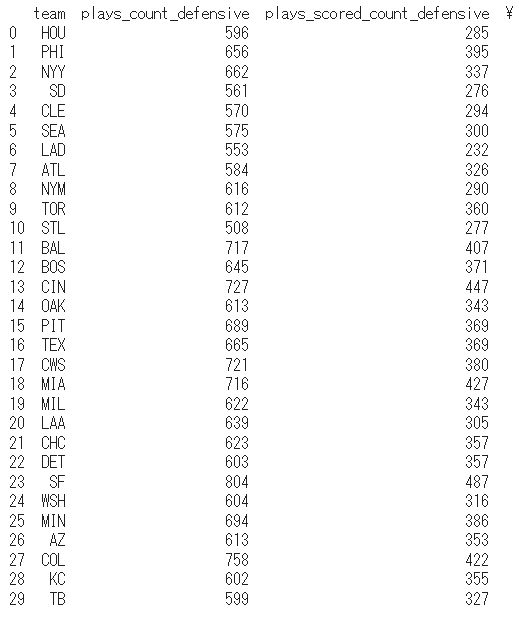
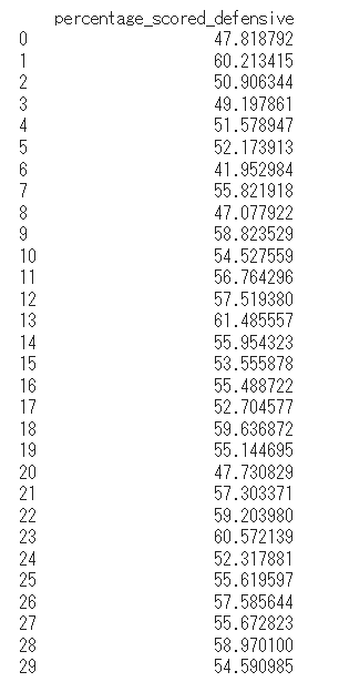
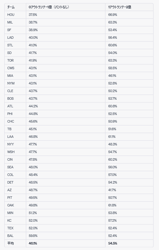
各チームの守備での失点割合

このコードは、各チームが守備側として1アウト2塁の状況で失点につながった割合を計算し、結果をデータフレームにまとめて表示します。

team_defensive_scores = []

for team in teams:
    # Filter for 1 out 2 base events for the team as the defensive team
    defensive_team_plays = df_filtered[((df_filtered['home_team'] == team) & (df_filtered['inning_topbot'] == 'Top')) | ((df_filtered['away_team'] == team) & (df_filtered['inning_topbot'] == 'Bot'))]
    
    # Calculate the percentage of plays that led to a run being scored
    percentage_scored_defensive_team = defensive_team_plays['inning_scored'].mean() * 100
    
    # Calculate the number of plays and the number of times they led to a run being scored
    plays_count_defensive = len(defensive_team_plays)
    plays_scored_count_defensive = defensive_team_plays['inning_scored'].sum()
    
    team_defensive_scores.append({
        'team': team,
        'plays_count_defensive': plays_count_defensive,
        'plays_scored_count_defensive': plays_scored_count_defensive,
        'percentage_scored_defensive': percentage_scored_defensive_team
    })

team_defensive_scores_df = pd.DataFrame(team_defensive_scores)

print(team_defensive_scores_df)

各チームの守備での失点割合(グラフ)

このコードは、各チームの守備側で1アウト2塁の状況から失点につながった割合を棒グラフで表示するものです。各チームは失点率の低い順に並べられています。

import matplotlib.pyplot as plt

sorted_defensive_df = team_defensive_scores_df.sort_values('percentage_scored_defensive', ascending=True)

# プロットの準備
fig, ax = plt.subplots(figsize=(15, 7))

# 棒グラフをプロットします。
ax.bar(sorted_defensive_df['team'], sorted_defensive_df['percentage_scored_defensive'], color='blue')

# 軸ラベルとタイトルを設定します。
ax.set_xlabel('Teams')
ax.set_ylabel('Score Percentage from 1 Out 2 Base (Defensive Team)')
ax.set_title('Score Percentage from 1 Out 2 Base by Team (Defensive) - Low to High')

# グラフを表示します。
plt.show()

0アウト1塁→1アウト2塁の効果(今回は備忘録,検証用)